Copy number calling pipeline¶

Each operation is invoked as a sub-command of the main script, cnvkit.py. A listing of all sub-commands can be obtained with cnvkit --help or -h, and the usage information for each sub-command can be shown with the --help or -h option after each sub-command name:

cnvkit.py -h
cnvkit.py antitarget -h

A sensible output file name is normally chosen if it isn’t specified, except in the case of the text reporting commands, which print to standard output by default, and the matplotlib-based plotting commands (not diagram), which will display the plots interactively on the screen by default.

batch¶

Run the CNVkit pipeline on one or more BAM files:

cnvkit.py batch Sample.bam -t Tiled.bed -a Background.bed -r Reference.cnn
cnvkit.py batch *.bam --output-dir CNVs/ -t Tiled.bed -a Background.bed -r Reference.cnn

With the -p option, process each of the BAM files in parallel, as separate subprocesses. The status messages logged to the console will be somewhat disorderly, but the pipeline will take advantage of multiple CPU cores to complete sooner.

cnvkit.py batch *.bam -d CNVs/ -t Tiled.bed -a Background.bed -r Reference.cnn -p 8

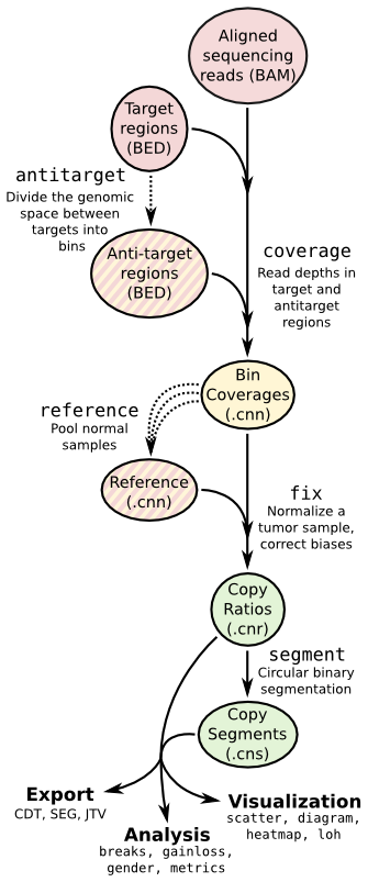
The pipeline executed by the batch command is equivalent to:

cnvkit.py coverage Sample.bam Tiled.bed -o Sample.targetcoverage.cnn
cnvkit.py coverage Sample.bam Background.bed -o Sample.antitargetcoverage.cnn
cnvkit.py fix Sample.targetcoverage.cnn Sample.antitargetcoverage.cnn Reference_cnn -o Sample.cnr
cnvkit.py segment Sample.cnr -o Sample.cns

See the rest of the commands below to learn about each of these steps and other functionality in CNVkit.

target¶

Prepare a BED file of baited regions for use with CNVkit.

cnvkit.py target Tiled.bed --annotate refFlat.txt --split -o Targets.bed

The BED file should be the baited genomic regions for your target capture kit, as provided by your vendor. Since these regions (usually exons) may be of unequal size, the --split option divides the larger regions so that the average bin size after dividing is close to the size specified by --average-size.

In case the vendor BED file does not label each region with a corresponding gene name, the --annotate option can add or replace these labels. Gene annotation databases, e.g. RefSeq or Ensembl, are available in “flat” format from UCSC (e.g. refFlat.txt for hg19).

In other cases the region labels are a combination of human-readable gene names and database accession codes, separated by commas (e.g. “ref|BRAF,mRNA|AB529216,ens|ENST00000496384”). The --short-names option splits these accessions on commas, then chooses the single accession that covers in the maximum number of consecutive regions that share that accession, and applies it as the new label for those regions. (You may find it simpler to just apply the refFlat annotations.)

If you need higher resolution, you can select a smaller average size for your target and antitarget bins.

Exons in the human genome have an average size of about 200bp. The target bin size default of 267 is chosen so that splitting larger exons will produce bins with a minimum size of 200. Since bins that contain fewer reads result in a noisier copy number signal, this approach ensures the “noisiness” of the bins produced by splitting larger exons will be no worse than average.

Setting the average size of target bins to 100bp, for example, will yield about twice as many target bins, which can result in more precise and perhaps more accurate segmentation. However, the number of reads counted in each bin will be reduced by about half, increasing the variance or “noise” in bin-level coverages. An excess of noisy bins can make visualization difficult, and since the noise may not be Gaussian, especially in the presence of many bins with zero reads, the CBS algorithm could produce less accurate segmentation results on low-coverage samples. In practice we see good results with an average of 200-300 reads per bin; we therefore recommend an overall on-target sequencing coverage depth of at least 200x to 300x with a read length of 100 to justify reducing the average target bin size to 100bp.

antitarget¶

Given a “target” BED file that lists the chromosomal coordinates of the tiled regions used for targeted resequencing, derive a BED file off-target/”antitarget”/”background” regions.

cnvkit.py antitarget Tiled.bed -g data/access-5kb-mappable.hg19.bed -o Background.bed

Many fully sequenced genomes, including the human genome, contain large regions of DNA that are inaccessable to sequencing. (These are mainly the centromeres, telomeres, and highly repetitive regions.) In the FASTA genome sequence these regions are filled in with large stretches of “N” characters. These regions cannot be mapped by resequencing, so we can avoid them when calculating the antitarget locations by passing the locations of the accessible sequence regions with the -g or --access option. These regions are precomputed for the UCSC reference human genome hg19 (data/access-5kb-mappable.hg19.bed), and can be computed for other genomes with the included script genome2access.py.

CNVkit uses a cautious default off-target bin size that, in our experience, will typically include more reads than the average on-target bin. However, we encourage the user to examine the coverage statistics reported by CNVkit and specify a properly calculated off-target bin size for their samples in order to maximize copy number information.

coverage¶

Calculate coverage in the given regions from BAM read depths.

With the -p option, calculates mean read depth from a pileup; otherwise, counts the number of read start positions in the interval and normalizes to the interval size.

cnvkit.py coverage Sample.bam Tiled.bed -o Sample.targetcoverage.cnn
cnvkit.py coverage Sample.bam Background.bed -o Sample.antitargetcoverage.cnn

Summary statistics of read counts and their binning are printed to standard error when CNVkit finishes calculating the coverage of each sample (through either the batch or coverage commands).

Note

The BAM file must be sorted. CNVkit (and most other software) will not notice out if the reads are out of order; it will just ignore the out-of-order reads and the coverages will be zero after a certain point early in the file (e.g. in the middle of chromosome 2). A future release may try to be smarter about this.

Note

If you’ve prebuilt the BAM index file (.bai), make sure its timestamp is later than the BAM file’s. CNVkit will automatically index the BAM file if needed – that is, if the .bai file is missing, or if the timestamp of the .bai file is older than that of the corresponding .bam file. This is done in case the BAM file has changed after the index was initially created. (If the index is wrong, CNVkit will not catch this, and coverages will be mysteriously truncated to zero after a certain point.) However, if you copy a set of BAM files and their index files (.bai) together over a network, the smaller .bai files will typically finish downloading first, and so their timestamp will be earlier than the corresponding BAM or FASTA file. CNVkit will then consider the index files to be out of date and will attempt to rebuild them. To prevent this, use the Unix command touch to update the timestamp on the index files after all files have been downloaded.

reference¶

Compile a copy-number reference from the given files or directory (containing normal samples). If given a reference genome (-f option), also calculate the GC content of each region.

cnvkit.py reference -o Reference.cnn -f ucsc.hg19.fa *targetcoverage.cnn

If normal samples are not available, it will sometimes work OK to build the reference from a collection of tumor samples. You can use the scatter command on the raw .cnn coverage files to help choose samples with relatively minimal CNVs for use in the reference.

Notes on sample selection:

You can use cnvkit.py metrics *.cnr -s *.cns to see if any samples are especially noisy. See the metrics command.
CNVkit will usually call larger CNAs reliably down to about 10x on-target coverage, but there will tend to be more spurious segments, and smaller-scale or subclonal CNAs can be hard to infer below that point. This is well below the minimum coverage thresholds typically used for SNV calling, especially for targeted sequencing of tumor samples that may have significant normal-cell contamination and subclonal tumor-cell populations. So, a normal sample that passes your other QC checks will probably be OK to use in building a CNVkit reference – assuming it was sequenced on the same platform as the other samples you’re calling.

Alternatively, you can create a “flat” reference of neutral copy number (i.e. log2 0.0) for each probe from the target and antitarget interval files. This still computes the GC content of each region if the reference genome is given.

cnvkit.py reference -o FlatReference.cnn -f ucsc.hg19.fa -t Tiled.bed -a Background.bed

Two possible uses for a flat reference:

Extract copy number information from one or a small number of tumor samples when no suitable reference or set of normal samples is available. The copy number calls will not be as accurate, but large-scale CNVs may still be visible.
Create a “dummy” reference to use as input to the batch command to process a set of normal samples. Then, create a “real” reference from the resulting *.targetcoverage.cnn and *.antitargetcoverage.cnn files, and re-run batch on a set of tumor samples using this updated reference.

Note

As with BAM files, CNVkit will automatically index the FASTA file if the corresponding .fai file is missing or out of date. If you have copied the FASTA file and its index together over a network, you may need to use the touch command to update the .fai file’s timestamp so that CNVkit will recognize it as up-to-date.

fix¶

Combine the uncorrected target and antitarget coverage tables (.cnn) and correct for biases in regional coverage and GC content, according to the given reference. Output a table of copy number ratios (.cnr).

cnvkit.py fix Sample.targetcoverage.cnn Sample.antitargetcoverage.cnn Reference.cnn -o Sample.cnr

segment¶

Infer discrete copy number segments from the given coverage table:

cnvkit.py segment Sample.cnr -o Sample.cns

By default this uses the circular binary segmentation algorithm (CBS), but with the -m option, the faster Fused Lasso algorithm (flasso) or even faster but less accurate HaarSeg algorithm (haar) can be used instead.

Fused Lasso additionally performs significance testing to distinguish CNAs from regions of neutral copy number, whereas CBS and HaarSeg by themselves only identify the supported segmentation breakpoints.

call¶

Given segmented log2 ratio estimates (.cns), round the copy ratio estimates to integer values using either:

A list of threshold log2 values for each copy number state, or
Some algebra, given known tumor cell fraction and normal ploidy.

cnvkit.py call Sample.cns -o Sample.call.cns
cnvkit.py call Sample.cns -y -m clonal --purity 0.65 -o Sample.call-clonal.cns
cnvkit.py call Sample.cns -y -m threshold -t=-1.1,-0.4,0.3,0.7 -o Sample.call-threshold.cns

The output is another .cns file, where the values in the log2 column are still log2-transformed, but represent integers in log2 scale – e.g. a neutral diploid state is represented as 0.0, not the integer 2. These output files are still compatible with the other CNVkit commands that accept .cns files, and can be plotted the same way.

The “clonal” method considers the observed log2 ratios in the input .cns file as a mix of some fraction of tumor cells (specified by --purity), possibly with altered copy number, and a remainder of normal cells with neutral copy number (specified by --ploidy for autosomes). This equation is rearranged to find the absolute copy number of the tumor cells alone, rounded to the nearest integer. The expected and observed ploidy of the sex chromosomes (X and Y) is different, so it’s important to specify -y/--male-reference if a male reference was used; the sample gender can be specified if known, otherwise it will be guessed from the log2 ratio of chromosome X.

The “threshold” method simply applies fixed log2 ratio cutoff values for each integer copy number state. This method therefore does not require the tumor cell fraction or purity to be known. The default cutoffs are reasonable for a tumor sample with purity of at least 40% or so; for germline samples, the -t values shown above may yield more accurate calls.