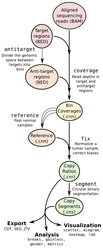
Copy number calling pipeline
Each operation is invoked as a sub-command of the main script, cnvkit.py.
A listing of all sub-commands can be obtained with cnvkit --help or -h,
and the usage information for each sub-command can be shown with the --help
or -h option after each sub-command name:
cnvkit.py -h
cnvkit.py target -h
A sensible output file name is normally chosen if it isn’t specified, except in
the case of the text reporting commands, which print to standard output by
default, and the matplotlib-based plotting commands (not diagram), which
will display the plots interactively on the screen by default.
batch
Run the CNVkit pipeline on one or more BAM files:
# From baits and tumor/normal BAMs
cnvkit.py batch *Tumor.bam --normal *Normal.bam \
    --targets my_baits.bed --annotate refFlat.txt \
    --fasta hg19.fasta --access data/access-5kb-mappable.hg19.bed \
    --output-reference my_reference.cnn --output-dir results/ \
    --diagram --scatter

# Reusing a reference for additional samples
cnvkit.py batch *Tumor.bam -r Reference.cnn -d results/

# Reusing targets and antitargets to build a new reference, but no analysis
cnvkit.py batch -n *Normal.bam --output-reference new_reference.cnn \
    -t my_targets.bed -a my_antitargets.bed \
    -f hg19.fasta -g data/access-5kb-mappable.hg19.bed
With the -p option, process each of the BAM files in parallel, as separate
subprocesses. The status messages logged to the console will be somewhat
disorderly, but the pipeline will take advantage of multiple CPU cores to
complete sooner.
cnvkit.py batch *.bam -r my_reference.cnn -p 8
The pipeline executed by the batch command is equivalent to:
cnvkit.py access baits.bed --fasta hg19.fa -o access.hg19.bed
cnvkit.py autobin *.bam -t baits.bed -g access.hg19.bed [--annotate refFlat.txt --short-names]

# For each sample...
cnvkit.py coverage Sample.bam baits.target.bed -o Sample.targetcoverage.cnn
cnvkit.py coverage Sample.bam baits.antitarget.bed -o Sample.antitargetcoverage.cnn

# With all normal samples...
cnvkit.py reference *Normal.{,anti}targetcoverage.cnn --fasta hg19.fa -o my_reference.cnn

# For each tumor sample...
cnvkit.py fix Sample.targetcoverage.cnn Sample.antitargetcoverage.cnn my_reference.cnn -o Sample.cnr
cnvkit.py segment Sample.cnr -o Sample.cns

# Optionally, with --scatter and --diagram
cnvkit.py scatter Sample.cnr -s Sample.cns -o Sample-scatter.pdf
cnvkit.py diagram Sample.cnr -s Sample.cns -o Sample-diagram.pdf
This is for hybrid capture protocols in which both on- and off-target reads can
be used for copy number detection. To run alternative pipelines for targeted
amplicon sequencing or whole genome sequencing, use the --method option with
value amplicon or wgs, respectively. The default is hybrid.
See the rest of the commands below to learn about each of these steps and other functionality in CNVkit.
target
Prepare a BED file of baited regions for use with CNVkit.
cnvkit.py target my_baits.bed --annotate refFlat.txt --split -o my_targets.bed
The BED file should be the baited genomic regions for your target capture kit,
as provided by your vendor. Since these regions (usually exons) may be of
unequal size, the --split option divides the larger regions so that the
average bin size after dividing is close to the size specified by
--average-size. If any of these three (--split, --annotate, or
--short-names) flags are used, a new target BED file will be created;
otherwise, the provided target BED file will be used as-is.
Bin size and resolution
If you need higher resolution, you can select a smaller average size for your target and antitarget bins.
Exons in the human genome have an average size of about 200bp. The target bin size default of 267 is chosen so that splitting larger exons will produce bins with a minimum size of 200. Since bins that contain fewer reads result in a noisier copy number signal, this approach ensures the “noisiness” of the bins produced by splitting larger exons will be no worse than average.
Setting the average size of target bins to 100bp, for example, will yield about twice as many target bins, which might result in higher-resolution segmentation. However, the number of reads counted in each bin will be reduced by about half, increasing the variance or “noise” in bin-level coverages. An excess of noisy bins can make visualization difficult, and since the noise may not be normally distributed, especially in the presence of many bins with zero reads, the segmentation algorithm could produce less accurate results on low-coverage samples. In practice we see good results with an average of 200–300 reads per bin; we therefore recommend an overall on-target sequencing coverage depth of at least 200x to 300x with a read length of 100bp to justify reducing the average target bin size to 100bp.
For hybrid capture, if your targets are not tiled with uniform density – for example, if your target panel is designed with a subset of targets having twice or half the usual number of tiles for a fixed number of genomic bases – you do not need to do anything in particular to compensate for this as long as you are using a pooled reference. When a test sample’s read depths are normalized to the pooled reference, the log2 ratios will even out. However, the “spread” of those bins in your pooled reference, and the “weight” of the corresponding bins in the test sample’s .cnr file, will be correspondingly higher or lower.
If some targets are enriched separately for each sample via spike-in, rather
than as part of the original capture panel (which is assumed to have a fairly
consistent capture efficiency across targets for all test and control samples),
then the spike-in capture efficiency will typically vary too much to be useful
as a copy number signal. In that case, the spike-in region should not be
included in the target BED file, and excluded from the access regions
(which determine antitarget regions) by using the -x option.
Labeling target regions
In case the vendor BED file does not label each region with a corresponding gene
name, the --annotate option can add or replace these labels.
Gene annotation databases, e.g. RefSeq or Ensembl, are available in “flat”
format from UCSC (e.g. refFlat.txt for hg19).
In other cases the region labels are a combination of human-readable gene names
and database accession codes, separated by commas (e.g.
“ref|BRAF,mRNA|AB529216,ens|ENST00000496384”). The --short-names option
splits these accessions on commas, then chooses the single accession that covers
in the maximum number of consecutive regions that share that accession, and
applies it as the new label for those regions. (You may find it simpler to just
apply the refFlat annotations.)
The targets do not need to be genes, but for convenience CNVkit’s documentation and source code generally refer to consecutive targeted regions with the same label as “genes”.
access
Calculate the sequence-accessible coordinates in chromosomes from the given reference genome, output as a BED file.
cnvkit.py access hg19.fa -x excludes.bed -o access-excludes.hg19.bed
cnvkit.py access mm10.fasta -s 10000 -o access-10kb.mm10.bed
Many fully sequenced genomes, including the human genome, contain large regions of DNA that are inaccessable to sequencing. (These are mainly the centromeres, telomeres, and highly repetitive regions.) In the reference genome sequence these regions are filled in with large stretches of “N” characters. These regions cannot be mapped by resequencing, so CNVkit avoids them when calculating the antitarget bin locations.
The access command computes the locations of the accessible sequence regions
for a given reference genome based on these masked-out sequences, treating long
spans of ‘N’ characters as the inaccessible regions and outputting the
coordinates of the regions between them.
Other known unmappable, variable, or poorly sequenced regions can be
excluded with the -x/--exclude option.
This option can be used more than once to exclude several BED files listing
different sets of regions.
For example, regions of poor mappability have been precalculated by others and
are available from the UCSC FTP Server (see here for hg19).
If there are many small excluded/inaccessible regions in the genome, then small,
less-reliable antitarget bins would be squeezed into the remaining accessible
regions. The -s option ignores short regions that would otherwise be
excluded, allowing larger antitarget bins to overlap them.
An “access” file precomputed for the UCSC reference human genome build hg19,
with some know low-mappability regions excluded, is included in the CNVkit
source distribution under the data/ directory
(data/access-5kb-mappable.hg19.bed).
antitarget
Given a “target” BED file that lists the chromosomal coordinates of the tiled regions used for targeted resequencing, derive a BED file off-target/”antitarget” regions.
cnvkit.py antitarget my_targets.bed -g data/access-5kb-mappable.hg19.bed -o my_antitargets.bed
Certain genomic regions cannot be mapped by short-read resequencing (see
access); we can avoid them when calculating the antitarget locations by
passing the locations of the accessible sequence regions with the -g or
--access option. CNVkit will then compute “antitarget” bins only within the
accessible genomic regions specified in the “access” file.
CNVkit uses a cautious default off-target bin size that, in our experience, will typically include more reads than the average on-target bin. However, we encourage the user to examine the coverage statistics reported by CNVkit and specify a properly calculated off-target bin size for their samples in order to maximize copy number information.
Off-target bin size
An appropriate off-target bin size can be computed as the product of the average target region size and the fold-enrichment of sequencing reads in targeted regions, such that roughly the same number of reads are mapped to on– and off-target bins on average — roughly proportional to the level of on-target enrichment. The autobin command (below) can quickly estimate these values, but you are free to specify your own.
Average off-target coverage depths can also be obtained with the script CalculateHsMetrics in the Picard suite (http://picard.sourceforge.net/), or from the console output of the CNVkit coverage command when run on the target regions.
Note
The generated off-target bins are given the label “Antitarget” in CNVkit versions 0.9.0 and later. In earlier versions, the label “Background” was used – CNVkit will still accept this label for compatibility.
autobin
Quickly estimate read counts or depths in a BAM file to estimate reasonable on- and (if relevant) off-target bin sizes. If multiple BAMs are given, use the BAM with median file size.
Generates target and (if relevant) antitarget BED files, and prints a table of estimated average read depths and recommended bin sizes on standard output.
cnvkit.py autobin *.bam -t my_targets.bed -g access.hg19.bed
cnvkit.py autobin *.bam -m amplicon -t my_targets.bed
cnvkit.py autobin *.bam -m wgs -b 50000 -g access.hg19.bed --annotate refFlat.txt
The BAM index (.bai) is used to quickly determine the total number of reads
present in a file, and random sampling of targeted regions (-t) is used to
estimate average on-target read depth much faster than the coverage
command.
coverage
Calculate coverage in the given regions from BAM read depths.
By default, coverage is calculated via mean read depth from a pileup. Alternatively, using the –count option counts the number of read start positions in the interval and normalizes to the interval size.
cnvkit.py coverage Sample.bam targets.bed -o Sample.targetcoverage.cnn
cnvkit.py coverage Sample.bam antitargets.bed -o Sample.antitargetcoverage.cnn
Summary statistics of read counts and their binning are printed to standard error when CNVkit finishes calculating the coverage of each sample (through either the batch or coverage commands).
BAM file preparation
For best results, use an aligner such as BWA-MEM, with the option to mark secondary mappings of reads, and flag PCR duplicates with a program such as SAMBLASTER, SAMBAMBA, or the MarkDuplicates script in Picard tools, so that CNVkit will skip these reads when calculating read depth.
You will probably want to index the finished BAM file using samtools or SAMBAMBA. But if you haven’t done this beforehand, CNVkit will automatically do it for you.
Note
The BAM file must be sorted. CNVkit will check that the first few reads are sorted in positional order, and raise an error if they are not. However, CNVkit might not notice if reads later in the file are unsorted; it will just silently ignore the out-of-order reads and the coverages will be zero after that point. So be safe, and sort your BAM file properly.
Note
If you’ve prebuilt the BAM index file (.bai), make sure its timestamp is
later than the BAM file’s. CNVkit will automatically index the BAM file
if needed – that is, if the .bai file is missing, or if the timestamp
of the .bai file is older than that of the corresponding .bam file. This
is done in case the BAM file has changed after the index was initially
created. (If the index is wrong, CNVkit will not catch this, and coverages
will be mysteriously truncated to zero after a certain point.) However,
if you copy a set of BAM files and their index files (.bai) together over
a network, the smaller .bai files will typically finish downloading first,
and so their timestamp will be earlier than the corresponding BAM or FASTA
file. CNVkit will then consider the index files to be out of date and will
attempt to rebuild them. To prevent this, use the Unix command touch
to update the timestamp on the index files after all files have been
downloaded.
reference
Compile a copy-number reference from the given files or directory (containing normal samples). If given a reference genome (-f option), also calculate the GC content and repeat-masked proportion of each region.
The reference can be constructed from zero, one or multiple control samples (see below).
A reference should be constructed specifically for each target capture panel, using a BED file listing the genomic coordinates of the baited regions. Ideally, the control or “normal” samples used to build the reference should match the type of sample (e.g. FFPE-extracted or fresh DNA) and library preparation protocol or kit used for the test (e.g. tumor) samples.
For target amplicon or whole-genome sequencing protocols, the “antitarget” BED and .cnn files can be omitted. Otherwise, ensure the filename prefixes are the same for each pair of “.targetcoverage.cnn” and “.antitargetcoverage.cnn” files (as it’s done by default).
Paired or pooled normals
Provide the *.targetcoverage.cnn and *.antitargetcoverage.cnn files
created by the coverage command:
cnvkit.py reference *coverage.cnn -f ucsc.hg19.fa -o Reference.cnn
To analyze a cohort sequenced on a single platform, we recommend combining all normal samples into a pooled reference, even if matched tumor-normal pairs were sequenced – our benchmarking showed that a pooled reference performed slightly better than constructing a separate reference for each matched tumor-normal pair. Furthermore, even matched normals from a cohort sequenced together can exhibit distinctly different copy number biases (see Plagnol et al. 2012 and Backenroth et al. 2014); reusing a pooled reference across the cohort provides some consistency to help diagnose such issues.
Notes on sample selection:
- You can use
cnvkit.py metrics *.cnr -s *.cnsto see if any samples are especially noisy. See the metrics command. - CNVkit will usually call larger CNAs reliably down to about 10x on-target coverage, but there will tend to be more spurious segments, and smaller-scale or subclonal CNAs can be hard to infer below that point. This is well below the minimum coverage thresholds typically used for SNV calling, especially for targeted sequencing of tumor samples that may have significant normal-cell contamination and subclonal tumor-cell populations. So, a normal sample that passes your other QC checks will probably be OK to use in building a CNVkit reference – assuming it was sequenced on the same platform as the other samples you’re calling.
If normal samples are not available, it will sometimes be acceptable to build the
reference from a collection of tumor samples. You can use the scatter command
on the raw .cnn coverage files to help choose samples with relatively
minimal and non-recurrent CNVs for use in the reference.
With no control samples
Alternatively, you can create a “flat” reference of neutral copy number (i.e. log2 0.0) for each probe from the target and antitarget interval files. This still computes the GC content of each region if the reference genome is given.
cnvkit.py reference -o FlatReference.cnn -f ucsc.hg19.fa -t targets.bed -a antitargets.bed
Possible uses for a flat reference include:
- Extract copy number information from one or a small number of tumor samples when no suitable reference or set of normal samples is available. The copy number calls will not be quite as accurate, but large-scale CNVs should still be visible.
- Create a “dummy” reference to use as input to the
batchcommand to process a set of normal samples. Then, create a “real” reference from the resulting*.targetcoverage.cnnand*.antitargetcoverage.cnnfiles, and re-runbatchon a set of tumor samples using this updated reference. - Evaluate whether a given paired or pooled reference is suitable for an analysis by repeating the CNVkit analysis with a flat reference and comparing the CNAs found with both the original and flat reference for the same samples.
How it works
CNVkit uses robust methods to extract a usable signal from the reference samples.
Each input sample is first median-centered, then read-depth bias corrections (the same used in the fix command) are performed on each of the normal samples separately.
The samples’ median-centered, bias-corrected log2 read depth values are then combined to take the weighted average (Tukey’s biweight location) and spread (Tukey’s biweight midvariance) of the values at each on– and off-target genomic bin among all samples. (For background on these statistical methods see Lax (1985) and Randal (2008).) To adjust for the lower statistical reliability of a smaller number of samples for estimating parameters, a “pseudocount” equivalent to one sample of neutral copy number is included in the dataset when calculating these values.
These values are saved in the output “reference.cnn” file as the “log2” and “spread” columns, indicating the expected read depth and the reliability of this estimate.
If a FASTA file of the reference genome is given, for each genomic bin the
fraction of GC (proportion of “G” and “C” characters among all “A”, “T”, “G” and
“C” characters in the subsequence, ignoring “N” and any other ambiguous
characters) and repeat-masked values (proportion of lowercased non-“N”
characters in the sequence)
are calculated and stored in the output “reference.cnn” file as columns “gc” and
“rmask”.
For efficiency, the samtools FASTA index file (.fai) is used to locate the
binned sequence regions in the FASTA file.
If the GC or RepeatMasker bias corrections are skipped using the --no-gc or
--no-rmask options, then those columns are omitted from the output file; if
both are skipped, then the genome FASTA file (if provided) is not examined at
all.
The result is a reference copy-number profile that can then be used to correct other individual samples.
Note
As with BAM files, CNVkit will automatically index the FASTA file if the
corresponding .fai file is missing or out of date. If you have copied the
FASTA file and its index together over a network, you may need to use the
touch command to update the .fai file’s timestamp so that CNVkit will
recognize it as up-to-date.
fix
Combine the uncorrected target and antitarget coverage tables (.cnn) and correct for biases in regional coverage and GC content, according to the given reference. Output a table of copy number ratios (.cnr).
cnvkit.py fix Sample.targetcoverage.cnn Sample.antitargetcoverage.cnn Reference.cnn -o Sample.cnr
How it works
The “observed” on- and off-target read depths are each median-centered and bias-corrected, as when constructing the reference. The corresponding “expected” normalized log2 read-depth values from the reference are then subtracted for each set of bins.
Bias corrections use the GC and RepeatMasker information from the “gc” and
“rmask” columns of the reference .cnn file; if those are missing (i.e. the
reference was built without those corrections), fix will skip them too (with
a warning). If you constructed the reference but then called fix with a
different set of bias correction flags, the biases could be over- or
under-corrected in the test sample – so use the options --no-gc,
--no-rmask and --no-edge consistently or not at all.
CNVkit filters out bins failing certain predefined criteria: those where the reference log2 read depth is below a threshold (default -5), or the spread of read depths among all normal samples in the reference is above a threshold (default 1.0).
A weight is assigned to each remaining bin depending on:
- The size of the bin;
- The deviation of the bin’s log2 value in the reference from 0;
- The “spread” of the bin in the reference.
(The latter two only apply if at least one normal/control sample was used to build the reference.)
Finally, the corrected on- and off-target bin-level copy ratios with associated weights are concatenated, sorted, and written to a .cnr file.
segment
Infer discrete copy number segments from the given coverage table:
cnvkit.py segment Sample.cnr -o Sample.cns
Segmentation runs independently on each chromosome arm, and can be parallelized
with the -p option (except for flasso and the HMM methods), similar to
batch.
The significance threshold to accept a segment or breakpoint is passed to the
underlying method with the option --threshold/-t. This is typically the
p-value or q-value cutoff, or whatever parameter the underlying method uses to
adjust its sensitivity.
Segmentation methods
The following segmentation algorithms can be specified with the -m option:
cbs– the default, circular binary segmentation (CBS). This method performed best in our benchmarking on mid-size target panels and exomes. Depends on the R package DNAcopy.flasso– Fused Lasso, reported by some users to perform best on exomes, whole genomes, and some target panels. Signficantly faster than CBS, but the current implementation cannot be parallelized over multiple CPUs. Beyond identifying breakpoints, additionally performs significance testing to distinguish CNAs from regions of neutral copy number, so large swathes of the output may have log2 values of exactly 0. Depends on the R package cghFLasso.haar– a pure-Python implementation of HaarSeg, a wavelet-based method. Very fast and performs reasonably well on small panels, but tends to over-segment large datasets.hmm(experimental) – a 3-state Hidden Markov Model suitable for most samples. Faster than CBS, slower but more accurate than Haar. Depends on the Python package hmmlearn, as do the next two methods.hmm-tumor(experimental) – a 5-state HMM suitable for finer-grained segmentation of good-quality tumor samples. In particular, this method can detect focal amplifications within a larger-scale, smaller-amplitude copy number gain, or focal deep deletions within a larger-scale hemizygous loss. Training this model takes a bit more CPU time than the simplerhmmmethod.hmm-germline(experimental) – a 3-state HMM with fixed amplitude for the loss, neutral, and gain states corresponding to absolute copy numbers of 1, 2, and 3. Suitable for germline samples and single-cell sequencing of samples with mostly-diploid genomes that are not overly aneuploid.none– simply calculate the weighted mean log2 value of each chromosome arm. Useful for testing or debugging, or as a baseline for benchmarking other methods.
The first two methods use R internally, and to use them you will need to have R
and the R package dependencies installed (i.e. DNAcopy, cghFLasso). If you
installed CNVkit with conda as recommended, these should have been installed
for you automatically. If you installed the R packages in a nonstandard
location, you can specify this location with --rlibpath.
The HMM methods hmm, hmm-tumor and hmm-germline were introduced
provisionally in CNVkit v.0.9.2, and may change in future releases.
They depend on the Python package hmmlearn, which is not installed by
default. You can install the latest hmmlearn (ideally within a conda or
virtualenv environment) after installing the rest of CNVkit with the command:
pip install hmmlearn
The methods haar and none do not have any additional dependencies beyond
the basic CNVkit installation.
Bin filtering
Bins with a weight of 0 are dropped before segmentation. Additional filters:
--drop-low-coverage– drop bins with a read depth of 0 or very close to 0, i.e. a log2 value suggesting the same. Use with tumor samples.--drop-outliers– drop bins with log2 value too far from a rolling average, taking local variability into account. Applied by default.
SNP allele frequencies
If a VCF file is given with the
--vcf option (and accompanying options -i, -n, -z, and
--min-variant-depth, which work as in other commands), then after segmenting
log2 ratios, a second pass of segmentation will run within each log2-ratio-based
segment on the SNP allele frequencies loaded from the VCF.
See also Calling copy number gains and losses for suggestions on how to interpret and post-process the resulting segments.
call
Given segmented log2 ratio estimates (.cns), derive each segment’s absolute integer copy number using either:
- A list of threshold log2 values for each copy number state (
-m threshold), or rescaling - for a given known tumor cell fraction and normal ploidy, then simple rounding to the nearest integer copy number (-m clonal).
cnvkit.py call Sample.cns -o Sample.call.cns
cnvkit.py call Sample.cns -y -m threshold -t=-1.1,-0.4,0.3,0.7 -o Sample.call.cns
cnvkit.py call Sample.cns -y -m clonal --purity 0.65 -o Sample.call.cns
cnvkit.py call Sample.cns -y -v Sample.vcf -m clonal --purity 0.7 -o Sample.call.cns
The output is another .cns file, with an additional “cn” column listing each segment’s absolute integer copy number. This .cns file is still compatible with the other CNVkit commands that accept .cns files, and can be plotted the same way with the scatter, heatmap and diagram commands. To get these copy number values in another format, e.g. BED or VCF, see the export command.
With a VCF file of SNVs (-v/--vcf), the b-allele frequencies of SNPs in
the tumor sample are extracted and averaged for each segment:
cnvkit.py call Sample.cns -y -v Sample.vcf -o Sample.call.cns
The segment b-allele frequencies are also used to calculate major and minor allele-specific integer copy numbers (see below).
Alternatively, the -m none option performs rescaling, re-centering, and
extracting b-allele frequencies from a VCF (if requested), but does not add a
“cn” column or allele copy numbers:
cnvkit.py call Sample.cns -v Sample.vcf --purity 0.8 -m none -o Sample.call.cns
Transformations
If there is a known level of normal-cell DNA contamination in the analyzed tumor sample (see the page on tumor heterogeneity), you can opt to rescale the log2 copy ratio estimates in your .cnr or .cns file to remove the impact of this contamination, so the resulting log2 ratio values in the file match what would be observed in a completely pure tumor sample.
With the --purity option, log2 ratios are rescaled to the value that would
be seen a completely pure, uncontaminated sample. The observed log2 ratios in
the input .cns file are treated as a mix of some fraction of tumor cells
(specified by --purity), possibly with altered copy number, and a remainder
of normal cells with neutral copy number (specified by --ploidy for
autosomes; by default, diploid autosomes, haploid Y or X/Y depending on
reference sex). This equation is rearranged to find the absolute copy number
of the tumor cells alone, rounded to the nearest integer.
The expected and observed ploidy of the sex chromosomes (X and Y)
is different, so if the option -y / --male-reference /
--haploid-x-reference was used when constructing the reference,
it’s important to specify use the same option here.
The sample sex can be specified if known, otherwise it will be guessed
from the average log2 ratio of chromosome X. (See also: Chromosomal sex)
When a VCF file containing SNV calls for the same tumor sample (and optionally a
matched normal) is given using the -v/--vcf option, the b-allele
frequencies (BAFs) of the heterozygous, non-somatic SNVs falling within each
segment are mirrored, averaged, and listed in the output .cns file as an
additional “baf” column (using the same logic as export nexus-ogt).
If --purity was specified, then the BAF values are also rescaled.
The call command can also optionally re-center the log2 values, though
this will typically not be needed since the .cnr files are automatically
median-centered by the fix command when normalizing to a reference and
correcting biases. However, if the analyzed genome is highly aneuploid and
contains widespread copy number losses or gains unequally, the default median
centering may place copy-number-neutral regions slightly above or below the
expected log2 value of 0.0. To address such cases, alternative centering
approaches can be specified with the --center option:
cnvkit.py call -m none Sample.cns --center mode
Calling methods
After the above adjustments, the “threshold” and “clonal” methods calculate the absolute integer copy number of each segment.
The “clonal” method converts the log2 values to absolute scale using the given
--ploidy, then simply rounds the absolute copy number values to the nearest
integer. This method is reasonable for germline samples, highly pure tumor
samples (e.g. cell lines), or when the tumor fraction is accurately known and
specified with --purity.
The “threshold” method applies fixed log2 ratio cutoff values for each
integer copy number state. This approach can be an alternative to specifying
and adjusting for the tumor cell fraction or purity directly. However, if
--purity is specified, then the log2 values will still be rescaled before
applying the copy number thresholds.
The default threshold values are reasonably “safe” for a tumor sample with
purity of at least 30%.
The inner cutoffs of +0.2 and -0.25 are sensitive enough to detect a single-copy
gain or loss in a diploid tumor with purity (or subclone cellularity) as low as
30%.
But the outer cutoffs of -1.1 and +0.7 assume 100% purity, so a more extreme
copy number, i.e. homozygous deletion (0 copies) or multi-copy amplification (4+
copies), is only assigned to a CNV if there is strong evidence for it.
For germline samples, the -t values shown below (or -m clonal) may yield
more precise calls.
The thresholds map to integer copy numbers in order, starting from zero: log2 ratios up to the first threshold value are assigned a copy number 0, log2 ratios between the first and second threshold values get copy number 1, and so on.
| If log2 value is up to | Copy number |
| -1.1 | 0 |
| -0.4 | 1 |
| 0.3 | 2 |
| 0.7 | 3 |
| … | … |
For homogeneous samples of known ploidy, you can calculate cutoffs from scatch by log-transforming the integer copy number values of interest, plus .5 (for rounding), divided by the ploidy. For a diploid genome:
>>> import numpy as np
>>> copy_nums = np.arange(5)
>>> print(np.log2((copy_nums+.5) / 2)
[-2.         -0.4150375   0.32192809  0.80735492  1.169925  ]
Or, in R:
> log2( (0:4 + .5) / 2)
[1] -2.0000000 -0.4150375  0.3219281  0.8073549  1.1699250
For arbitrary purity and ploidy:
> purity = 0.6
> ploidy = 4
> log2( (1 - purity) + purity * (0:6 + .5) / ploidy )
[1] -1.0740006 -0.6780719 -0.3677318 -0.1124747  0.1043367  0.2927817  0.4594316
Allele frequencies and counts
If a VCF file is given using the -v/--vcf option, then for each segment
containing SNVs in the VCF, an average b-allele frequency (BAF) within that
segment is calculated, and output in the “baf” column.
Allele-specific integer copy number values are then inferred from the total copy
number and BAF, and output in columns “cn1” and “cn2”.
This calculation uses the same method as PSCBS:
total copy number is multiplied by the BAF, and rounded to the nearest integer.
Allelic imbalance, including copy-number-neutral loss of heterozygosity (LOH), is then apparent when a segment’s “cn1” and “cn2” fields have different values.
Filtering segments
New in version 0.8.0.
Finally, segments can be filtered according to several criteria, which may be combined:
- Integer copy number (
cn), merging adjacent with the same called value. - Keeping only high-level amplifications (5 copies or more) and homozygous
deletions (0 copies) (
ampdel). - Confidence interval overlapping zero (
ci). - Standard error of the mean (
sem), a parametric estimate of confidence intervals which behaves similarly.
In each case, adjacent segments with the same value according to the given criteria are merged together and the column values are recalculated appropriately. Segments on different chromosomes or with different allele-specific copy number values will not be merged, even if the total copy number is the same.